Influencer or Observer: Predicting Social Roles
Kaggle challenge · CSC 51054, École Polytechnique · Autumn 2025 · with Joel Tagne Waffo & Sylvain Dehayem Kenfouo
Overview
Given a tweet and its account metadata, is the author an Influencer — someone who shapes opinions and drives engagement — or an Observer? This binary classification challenge came with a heterogeneous dataset mixing numerical metadata, categorical attributes, and raw tweet text, and we built the pipeline end to end: exploratory analysis, data preprocessing, feature engineering, LLM-based text encoders, gradient-boosted classifiers, hyperparameter tuning, and a final bagging ensemble that reached 0.859 accuracy on the leaderboard, placing us in the top 3 out of 120 teams.
Data analysis & preprocessing
The raw data had 192 features, and 73% of them were missing for more than half the rows. We dropped features with zero variance (they carry no signal) and those with more than 90% missing values.
The most valuable discovery of the whole project came from plain data analysis, not modelling: the dataset description mentions ~38k users, but user.created_at takes only ~30k distinct values — and all tweets sharing a creation date share the same label and nearly identical user metadata. Account creation timestamps are precise enough to act as a de facto user identifier. We therefore grouped tweets by user.created_at and imputed missing values within each group (median for numerical features, most frequent value otherwise), which denoises the data far better than global imputation.
Feature engineering
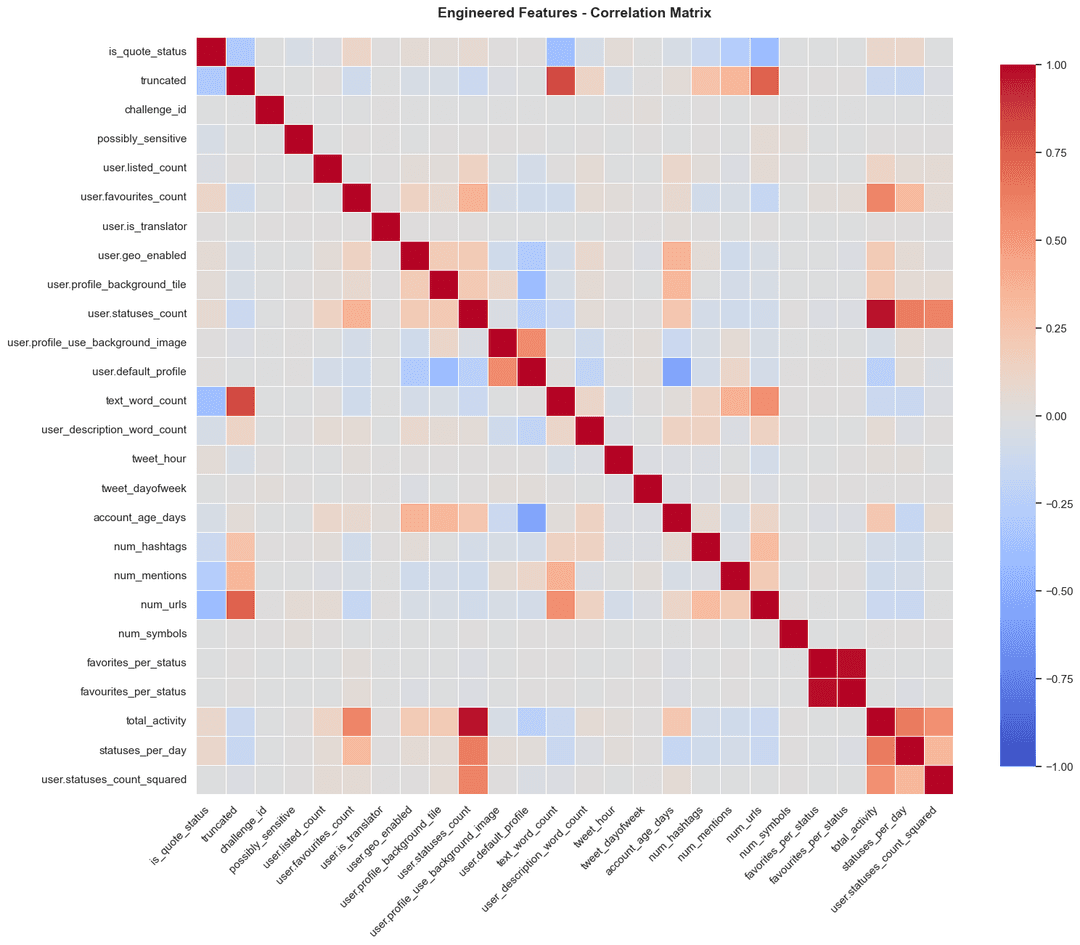
We built features at two levels, then aggregated everything to the user level. From the raw metadata we derived interpretable quantities:
plus activity rates (statuses_per_day, followers_per_day), text statistics (tweet length and word count, profile-description length), and temporal patterns (tweet hour and day of week). Averaging these per user — mean_user_listed, mean_total_activity, mean_tweet_hour, and so on — produced the features that consistently ranked at the top of the importance charts: a user's habits predict their role better than any single tweet.
Text encoders
To use the tweet text itself, we compared a spectrum of encoders, from TF-IDF to fine-tuned language models. Encoder-only models (BERT, RoBERTa, BERTweet) were fine-tuned for binary classification, and we then extracted their [CLS] embedding as a feature vector. We also tried LoRA fine-tuning, which freezes the pretrained weights W and learns only a low-rank update:
Pythia-160M, a decoder-only (GPT-like) model, was instead fine-tuned autoregressively on a prompt formulation:
What type of Twitter account posted this tweet?
{combined_text}
OPTIONS:
0: Observer
1: Influencer
ANSWER: {label}
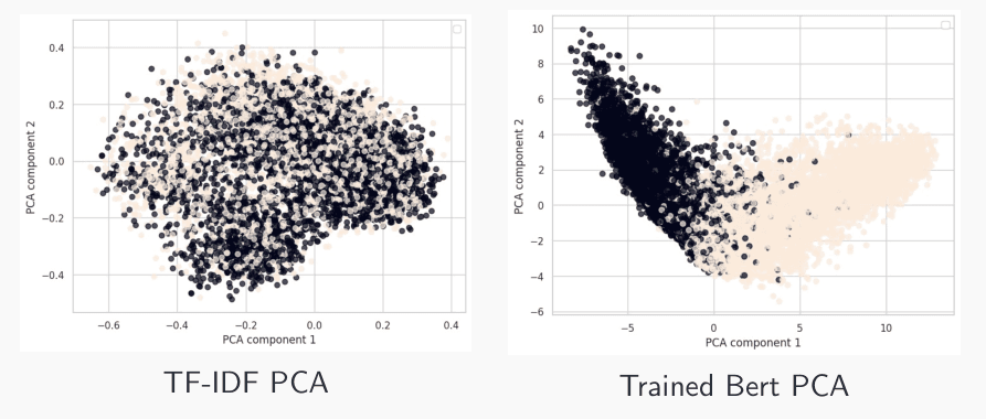
with its embedding taken as a mean-pool of the last hidden layer over non-padding tokens. Why go to that trouble? A PCA projection of the two extremes makes the answer visible:
Model pipeline
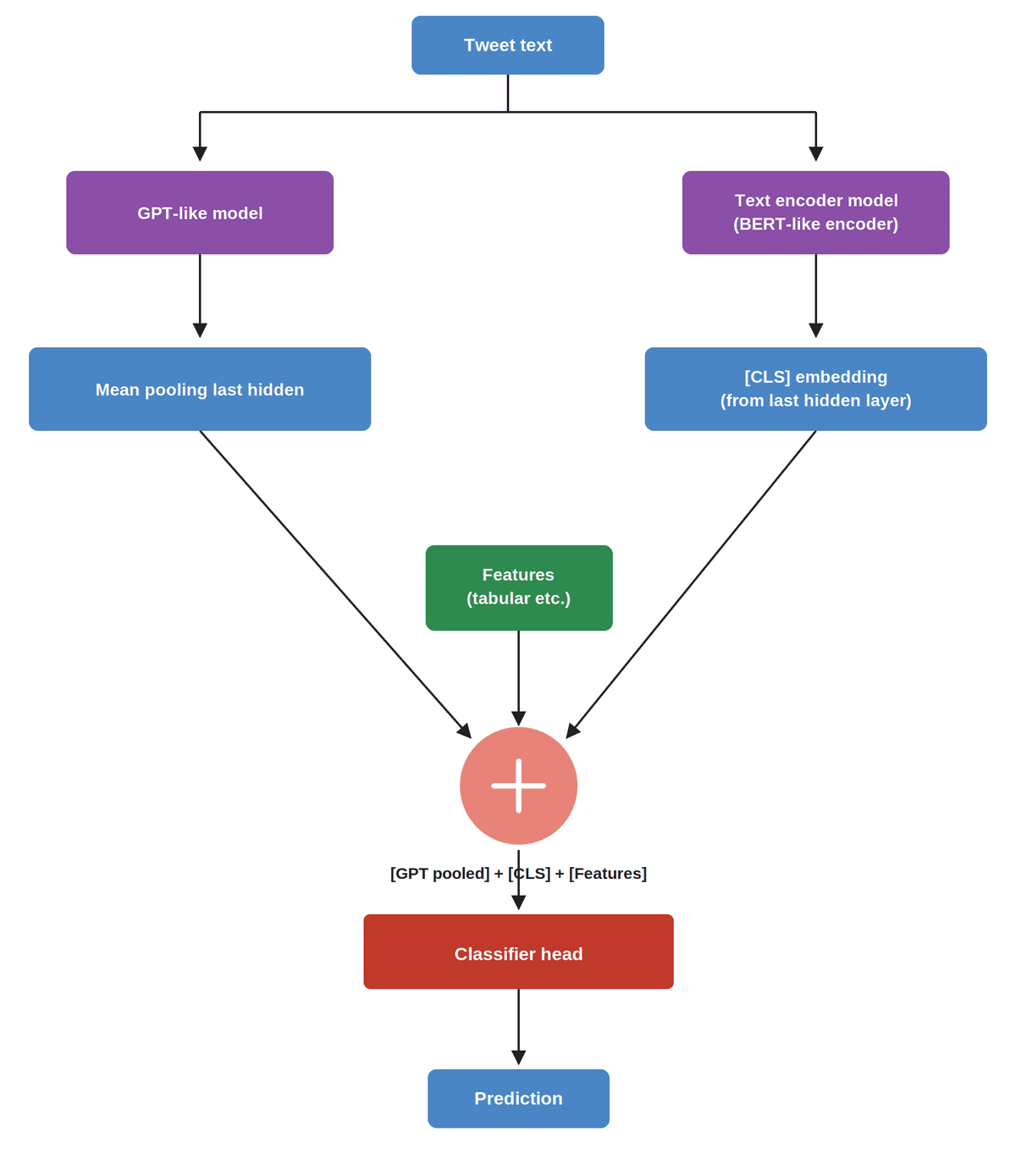
Each tweet ends up represented as the concatenation of the GPT-like pooled embedding, the BERT-like [CLS] embedding, and the engineered tabular features, fed into a classifier head. We compared an MLP, random forest, LightGBM, and XGBoost — the gradient-boosted trees won, with LightGBM matching XGBoost's accuracy at a fraction of the training time.
Hyperparameters (learning rate, tree depth, number of leaves, regularization) were tuned with Optuna, which samples promising configurations adaptively instead of exhaustively grid-searching — each trial scored by 5-fold cross-validation. Crucially, all splits used StratifiedGroupKFold at the user level: tweets from one user never appear in both train and validation folds, which would leak the (user-constant) label.
Ensembling
Three layers of averaging turn the base models into a robust predictor:
1. Cross-validation bagging. Each configuration is trained on 5 user-level folds, and the test-set probabilities are averaged over the folds:
2. User-level aggregation. Predictions are then made uniform per user (majority vote over a user's tweets) — since the label is a property of the user, not the tweet, this removes tweet-level noise and was one of the largest single score jumps.
3. Majority vote across decorrelated models. Finally, the strongest complementary configurations vote:
Bagging only helps when the models make different errors, and the feature-importance charts prove ours do:
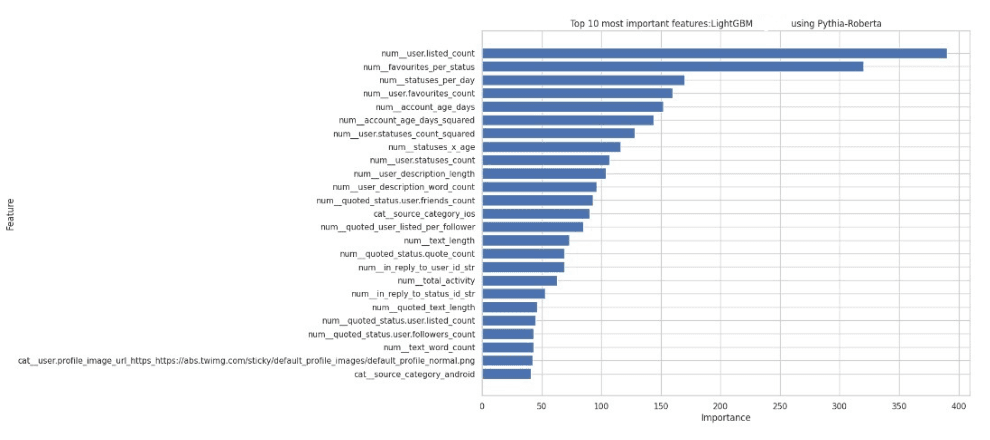
Remark. Every top feature here is behavioral, and the ranking is interpretable on its face. The strongest predictor, user.listed_count, counts how many public lists other people have added the account to — notoriety conferred by others, which is close to the definition of an influencer. Next come favourites_per_status and statuses_per_day: engineered ratios outranking the raw counts they were built from, confirming that normalizing activity by time or volume adds signal. Account age and its squared term also rank highly — influence correlates with how long an account has existed. Notably, RoBERTa and Pythia embedding dimensions were available to this model, yet almost none crack the top 25.
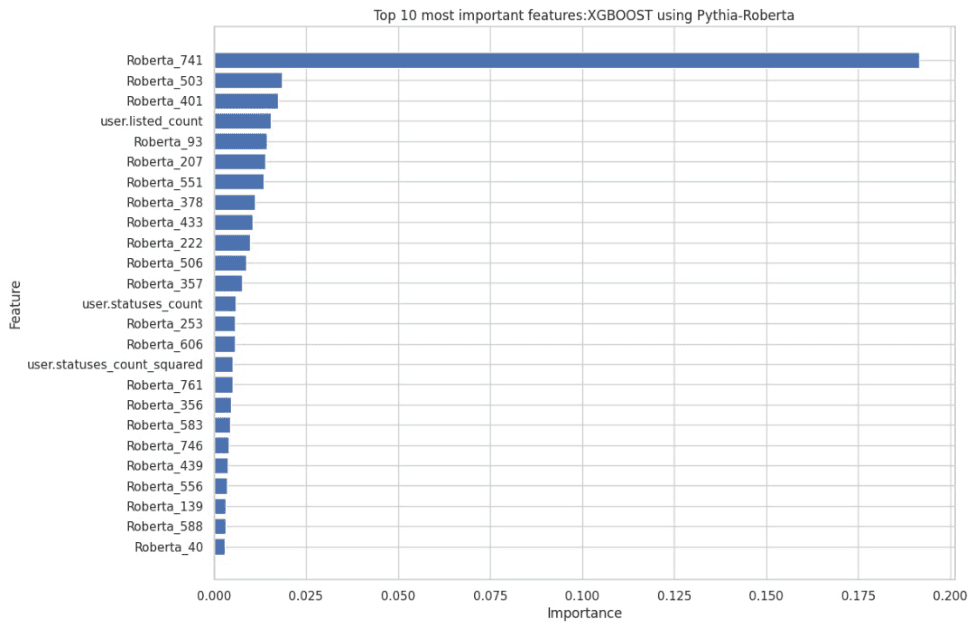
Remark. The picture inverts: the top of the ranking is almost entirely RoBERTa embedding dimensions, with Roberta_741 towering over everything else — the fine-tuned encoder has concentrated the class signal into a handful of directions of its embedding space. Individual dimensions aren't human-readable, but their dominance means this model decides mostly from the content and style of the text. Only a few metadata features (user.listed_count, user.statuses_count) survive in the ranking.
The two rankings barely overlap: one model reads the metadata, the other reads the text. Their errors are therefore weakly correlated — exactly the condition under which averaging reduces variance, and the empirical justification for the majority vote above.
Results
| Model | Accuracy |
|---|---|
| XGB + RoBERTa 2k + Pythia 6k | 0.845 |
| XGB + RoBERTa 0k + Pythia 6k | 0.845 |
| XGB + BERT LoRA fine-tuning | 0.843 |
| LGBM + RoBERTa 2k + Pythia 6k | 0.846 |
| LGBM + RoBERTa 3k + Pythia 6k (with user features) | 0.856 |
| LGBM + RoBERTa 0k + Pythia 6k | 0.846 |
| LGBM + RoBERTa 0k + Pythia 6k (with user features) | 0.852 |
| LGBM + RoBERTa 2k | 0.843 |
| LGBM + RoBERTa 2k (with user features) | 0.853 |
| LGBM + Pythia 0k | 0.840 |
| LGBM + TF-IDF (with user features) | 0.850 |
| LGBM + BERT LoRA fine-tuning | 0.843 |
| LGBM + BERTweet 0k + Pythia 6k (with user features) | 0.853 |
| Final ensemble — LGBM + XGBoost (RoBERTa 3k + Pythia 6k + BERTweet 0k) | 0.859 |
Two patterns stand out. Adding aggregated user features lifts every configuration by roughly a full point (0.846 → 0.856 for the best LightGBM) — feature engineering beat model swaps. And the ensemble adds a final, modest-but-consistent gain over the best single model (0.856 → 0.859), exactly what bagging theory predicts when averaging strong, partially decorrelated predictors.
Takeaways & future work
LLM embeddings carry real signal, but they paid off only when combined with disciplined tabular feature engineering and leak-free, user-level validation — the unglamorous parts of the pipeline drove most of the score. For future work: cheaper fine-tuning (LoRA, distilled models) to cut the dominant compute cost, and graph neural networks over the explicit social graph (followers, friends, mentions), since influence is ultimately a relational property that per-user features can only approximate.