Statistical Modelling of Random Processes: Three Case Studies

Three self-contained studies, one common thread: using stochastic processes and statistical inference to describe, forecast, and exploit complex dynamics in real data. The first forecasts the volatility of gold futures with a GARCH model; the second models crime contagion in Chicago with spatio-temporal Hawkes processes; the third captures the joint behaviour of two volatility indices with copulas and turns it into a profitable pair-trading strategy.

Gold is the classic safe-haven asset, and in a period marked by geopolitical tensions its price moves matter. Using daily data for the gold futures contract (GC=F) from Yahoo Finance, January 2025 to February 2026, we set out to forecast its volatility for March 2026.

Remark. The two panels justify the whole modelling strategy. The price (left) trends strongly upward — clearly non-stationary, confirmed by an ADF test that cannot reject a unit root. The log-returns (right) hover around zero with no trend — stationary — but the size of the swings is anything but constant: quiet stretches alternate with bursts like the sharp drop in early 2026. That combination — no structure in the mean (Ljung-Box tests find no significant autocorrelation), fat-tailed distribution (Jarque-Bera strongly rejects normality), but clustered variance — is the textbook signature calling for a GARCH model with Student-t innovations rather than any model of the returns themselves.

We fitted a GARCH(1,1) with Student-t innovations by maximum likelihood. All parameters came out statistically significant, and their values tell a coherent story: the volatility reacts noticeably to recent shocks, and above all it is highly persistent — the persistence terms sum to roughly 0.95, meaning a burst of volatility takes a long time to die out. The model was then used in a rolling one-step-ahead scheme (re-estimated at each date on 290 training observations, evaluated on 15 out-of-sample days) to forecast March 2026, giving a mean squared error of 0.898 in-sample and 1.36 out-of-sample.

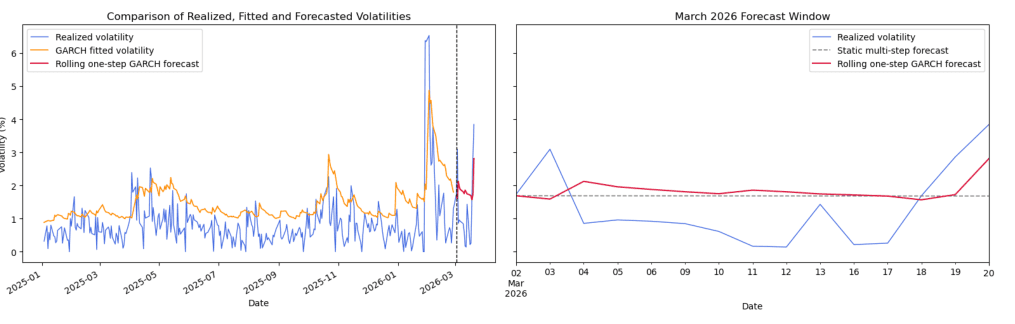
Remark. The fitted volatility (orange, left panel) tracks the level and the clustering of realized volatility well — including the large spike in early 2026 — but is visibly smoother: it rises with a short delay and undershoots the sharpest peaks. The zoom on March 2026 (right) shows why the rolling forecast (red) beats the static one (dashed): by re-estimating daily it bends toward the late-month volatility pickup that the static forecast misses entirely. Underestimating sudden extreme spikes is a known, structural limit of a standard GARCH(1,1) — it models persistence, not surprises — and the out-of-sample error being larger than the in-sample one quantifies exactly that.

Criminology documents a robust empirical pattern called near-repeat victimization: right after a crime, the probability of another crime nearby — in space and in time — is elevated. That is precisely the behaviour of a self-exciting (Hawkes) point process, where each event temporarily raises the intensity of future events around it. We fitted a multivariate spatio-temporal Hawkes model to the public Chicago crime registry for December 2015, restricted to two crime types: theft and battery. The model lets each type excite both itself and the other, with an exponentially decaying influence in time and a Gaussian-shaped influence in space.

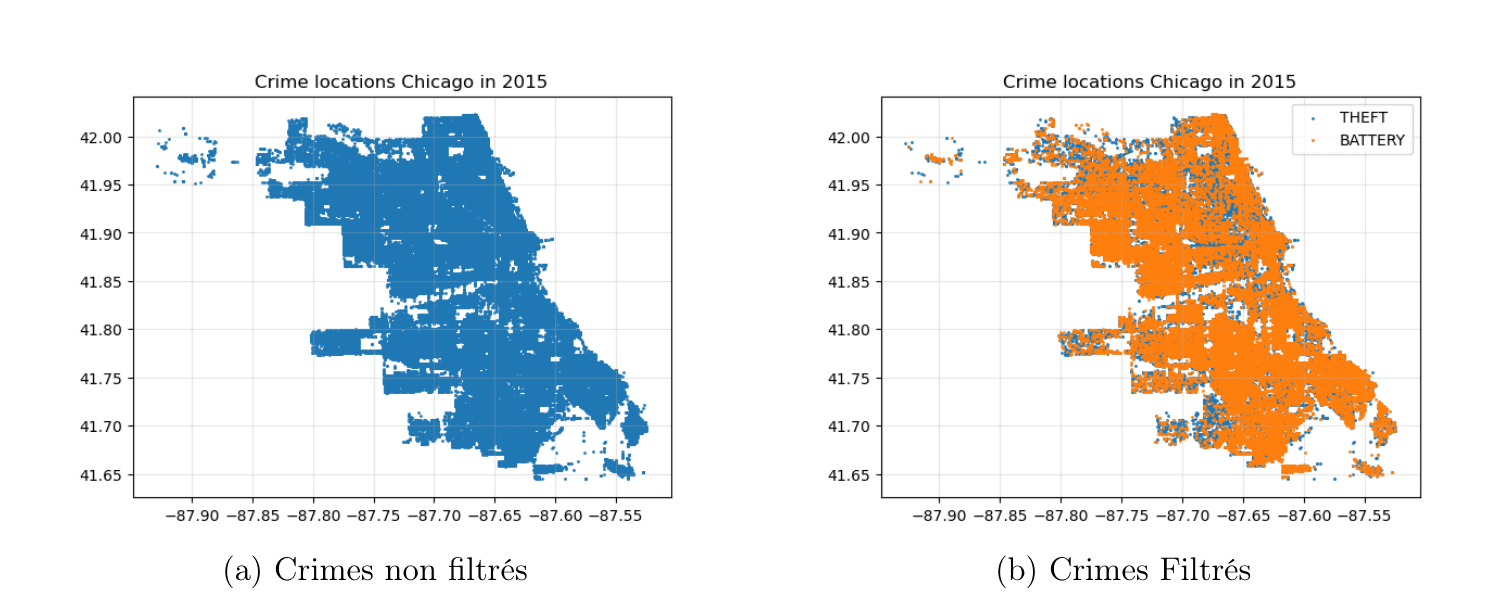
Remark. The point cloud is dense enough to redraw the city: the street grid, the empty airport corridor, the lakefront. Two practical lessons hide in this figure. First, the raw registry (left) needs real preprocessing before a point-process model can touch it — timestamps rounded to the minute create duplicated event times (fixed by adding a tiny random jitter), and latitude/longitude must be projected to kilometres (Lambert conformal projection), because the spatial kernel reasons in Euclidean distance. Second, the filtered map (right) shows theft and battery interleaved in the same neighbourhoods rather than occupying separate zones — spatial overlap that makes cross-excitation between the two types plausible before any parameter is estimated.

The eight model parameters were estimated by maximizing the point-process likelihood with L-BFGS-B, using five random restarts — the restarts landed on visibly different optima, so the multi-start strategy genuinely mattered. The fitted model is strikingly interpretable:

• the influence of a crime decays with a half-life of about 12.5 hours and a spatial range of about 0.8 km — an elevated risk lasting roughly a day, within walking distance;
• self-excitation dominates: a theft generates on average ~0.76 follow-up thefts, a battery ~0.64 follow-up batteries, while the cross effects (theft→battery, battery→theft) are smaller but far from negligible at ~0.24–0.25;
• the estimated background rates are tiny, and the branching ratios approach 1 (0.995 for theft, 0.892 for battery): almost every crime in the model is triggered by an earlier one rather than arising spontaneously, putting the system close to the critical regime where long cascades of events occur.

The VIX and RVX indices measure the implied volatility of US large-cap (S&P 500) and small-cap (Russell 2000) stocks. They spike together in every market stress episode, yet their relative level keeps drifting — which raises a trading question: when one of them is abnormally high given the level of the other, will the gap close? Copulas are the right tool for that question, because they model the dependence structure between two series separately from each series' own distribution.

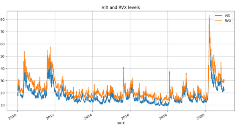
Remark. The two indices are almost mirror images — log-return correlation of 0.92 — and every spike is shared, from the 2011 and 2018 sell-offs to the huge COVID spike of March 2020. But look at the gap between the curves: RVX sits persistently above VIX, and the spread widens and narrows over time. That is the structure the strategy will exploit: strong co-movement makes a long/short position hedged against market-wide volatility shocks, while the fluctuating spread provides the mispricings to trade. The heavy tails visible in these series also explain why Student-t distributions beat the normal for both margins (by AIC/BIC and Kolmogorov–Smirnov tests).

After fitting the margins, we compared seven copula families by maximum likelihood on 2010–2020 data. The N14 copula — one with upper-tail dependence, fitting the tendency of both indices to explode together — won by a clear AIC margin over the Gaussian. The strategy then works on a rolling basis: margins and copula re-estimated on a 500-day window, and at each date the model produces the conditional probability that each index is unusually low or high given the other. When one index sits in an extreme conditional quantile (beyond 0.90), the strategy opens the corresponding long/short pair and closes it once the imbalance fades (back within 0.65) — with positions lagged one day to rule out look-ahead bias.

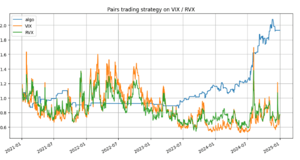
Remark. Over 2021–2025, simply holding either index lost about a third of its value — volatility indices decay in calm markets, so the benchmarks drift down (orange, green). The pair-trading strategy (blue) tells a different story: long flat stretches — it is out of the market most of the time, trading only when the copula flags a genuine imbalance — punctuated by steady gains and a strong acceleration from 2023 on. Final tally: +93.1% total return, 17.9% annualized, a Sharpe ratio of 0.88, and a maximum drawdown of −21.8%, versus drawdowns above 60% for the directional positions. Honest caveats remain: fixed unit weights with no dynamic hedge ratio, and no transaction costs in this first version — both would trim the numbers, neither erases the gap to the benchmarks.

Three datasets, three model families — conditional heteroskedasticity, self-exciting point processes, copulas — but one workflow throughout: diagnose the data's statistical properties first, choose the stochastic model those diagnostics call for, estimate it by maximum likelihood under real numerical constraints, and validate out of sample. The projects also share a failure-awareness: GARCH underestimates sudden spikes, the Hawkes likelihood landscape is multimodal, and the trading backtest ignores costs — knowing where a model stops working is part of the modelling.